Against the literature¶

The Verification page states, in numbers, how far the shipped tables sit from published references. This page shows the same comparisons as curves, for two representative elements — silicon and iron — so that the shape of the agreement is visible: where the calculations coincide, where they part, and how fast. It is written to be read without the Verification page first; the physics terms it needs are introduced as they come.

What is being compared, and against what¶

Three quantities, from the two published datasets:

Quantity	Dataset	Reference(s)	Kind of reference
X-ray scattering factor \(f_x(s)\)	dataset-factors v1.0.0	OFFV1 (Olukayode et al., 2023); Waasmaier & Kirfel (1995); Cromer & Mann (1968)	one computed table, two fits
Electron scattering factor \(f_e(s)\)	dataset-factors v1.0.0	OFFV1 through Mott–Bethe; Kirkland (2010); Peng et al. (1996)	one computed table, two fits
Ionization form factor \(F(s, E_0)\)	dataset v5.0.0	Oxley & Allen (2000); the µSTEM shape factors (Allen et al., 2015)	two computed shape tables

Two things to hold on to before looking at any panel:

A computed table is not a fit. OFFV1 is a set of numbers produced by an atomic-structure calculation (Dirac–Hartree–Fock) at 62 values of \(s\); agreeing with it means agreeing with that physics. Waasmaier–Kirfel, Cromer–Mann, Peng and Kirkland are fits — compact formulas (sums of Gaussians, or Gaussians plus Lorentzians) adjusted to reproduce a Hartree–Fock atom (a relativistic one for the more recent fits) over a stated range of \(s\). A fit carries its own residual against the numbers it was fitted to, and outside its range it is not a statement about the atom at all. So when a fit departs from the computed table at large \(s\) below, that is a property of the formula, not of the underlying physics — and agreeing with a fit can never say more than "within the fit's own residual".

Agreement with a calculation is not agreement with experiment. Every reference here is itself a calculation. What the panels test is whether Temari reproduces the physics those calculations contain — and, where it does not, how much and where. Correlation, chemical bonding and solid-state effects are absent from all of them alike.

Every figure plots a ratio or a relative deviation, never the reference values themselves. The published tables, the fitted coefficients and the output of GPL-licensed codes do not enter this repository in any form (see CONTRIBUTING); a deviation figure characterises the comparison without republishing anyone's work. Everything here is generated by one script, tools/make_comparison_figures.py, from the shipped tables and locally held copies of the references.

The three quantities in one paragraph each¶

\(f_x(s)\), the X-ray atomic scattering factor, is the Fourier transform of the atom's electron density: \(f_x(0) = Z\) (the electron count), and it falls as \(s\) grows because the density has finite extent. Units: electrons.
\(f_e(s)\), the electron scattering factor, is what a fast electron sees — the nucleus and the electron cloud together. The Mott–Bethe relation gives it from \(f_x\): \(f_e = (Z - f_x)/(8\pi^2 a_0 s^2)\). Near \(s = 0\) the numerator \(Z - f_x\) is a small difference of two large numbers, set by the second radial moment of the density (\(f_e(0) = a_0 M_2/3\)), so \(f_e\) near \(s = 0\) magnifies small differences in the outer density that \(f_x\) hides. Units: Å. Convention: first Born, without the incident electron's relativistic factor γ — the same as Doyle & Turner (1968) and Peng et al. (1996).
\(F(s, E_0)\), the inner-shell ionization form factor, is a different kind of quantity: it describes how the ionization of one subshell (Fe 1s, say) by an electron of energy \(E_0\) is distributed in momentum transfer, normalized to \(F(0) = 1\). It is signed, it depends on \(E_0\), and it is neither \(f_x\), nor \(f_e\), nor a cross section — see Data.

Throughout, \(s = \sin\theta/\lambda\) in Å⁻¹ (\(q = 4\pi s\)).

How to read a ratio panel

The vertical axis is \(100 \times (\text{Temari}/\text{reference} - 1)\) in percent — or, for the fits, \(100 \times (\text{fit}/\text{reference} - 1)\) — and the dashed line at zero is the reference. A curve at +1 % is one percent above the reference there. Where a curve leaves the frame it is cut, not clamped, and a label says where it went.

Two cautions. A ratio magnifies small absolute residuals where the factor itself is small (large \(s\) for \(f_x\), and near a zero crossing for the signed \(F\)), so the text gives absolute numbers where that matters. And a ratio through a zero carries no information at all — the L-shell \(F\) panel stops before the sign change for that reason.

1. X-ray scattering factor f_x(s)¶

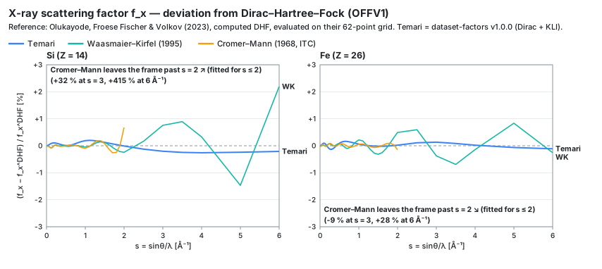
dataset-factors v1.0.0 (Dirac SCF with KLI exchange — the exchange-only KLI approximation to the optimized effective potential, OEP) is compared with the numerical Dirac–Hartree–Fock table OFFV1 (Olukayode et al., 2023) — a computed reference — and with the two analytic parameterizations everybody uses: Waasmaier & Kirfel (1995), five Gaussians plus a constant, fitted for \(s \le 6\) Å⁻¹; and Cromer & Mann (1968) as tabulated in the International Tables for Crystallography Vol. C (Prince, 2004), four Gaussians plus a constant, fitted for \(s \le 2\) Å⁻¹. All are evaluated on OFFV1's own 62-point grid — the reference is never interpolated; the shipped table is read at those nodes through its own contract spline (7681 nodes, an interpolation error far below anything visible here).

f_x of Si and Fe: relative deviation from DHF for Temari, Waasmaier–Kirfel and Cromer–Mann

What the figure shows:

Below \(s \approx 2\) Å⁻¹ every curve agrees with DHF to a fraction of a percent. Temari stays within 0.26 % (Si) and 0.17 % (Fe) of DHF over the whole range 0–6 Å⁻¹ — at most 0.011 e (Si) and 0.023 e (Fe) in absolute terms — because it is a calculation of the same physics (Dirac, exchange-only, correlation-free), not a fit to it.
Cromer–Mann leaves past \(s = 2\) Å⁻¹, its fit range: +32 % at \(s = 3\) and +415 % at \(s = 6\) for Si, −9 % and +28 % for Fe. This is the classic "agrees at small \(s\), departs at large \(s\)" pattern, and it is a property of the parameterization, not of the underlying Hartree–Fock atom it was fitted to.
Waasmaier–Kirfel holds to \(s = 6\) but oscillates by up to 0.24 % (Si) / 0.49 % (Fe) below \(s = 2\) and up to 2.2 % (Si) at the far end. That 2.2 % is 0.005 e — the fit's absolute residual — on an \(f_x\) that has fallen to 0.22 e.

The Verification page's RMS table (0.087 % / 0.079 % for Si / Fe over \(s \le 2\)) is the summary statistic of the Temari curves.

Take-away. For these atoms Temari follows exchange-only DHF to about a quarter of a percent (0.26 % / 0.17 %) over the whole range, and to under 0.1 % RMS below \(s = 2\); the fits are as good as their range and no further. Nothing here says anything about correlation or about experiment.

2. Electron scattering factor f_e(s)¶

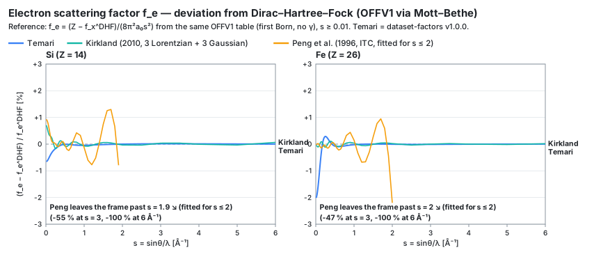
The same dataset, same reference. DHF has no separate \(f_e\) table, so the reference is derived from OFFV1 through the Mott–Bethe relation — the same first-Born, γ-free convention the shipped \(f_e\) uses — from OFFV1's first node \(s = 0.01\) onward. The literature curves are Kirkland's three-Lorentzian + three-Gaussian fit (Kirkland, 2010, Appendix C; fitted for \(s \le 6\) Å⁻¹ with a Lorentzian tail) and Peng et al. (1996) as tabulated in the International Tables Vol. C (Prince, 2004; five Gaussians, fitted for \(s \le 2\) Å⁻¹).

f_e of Si and Fe: relative deviation from DHF (via Mott–Bethe) for Temari, Kirkland and Peng

What the figure shows:

Peng leaves past \(s = 2\) Å⁻¹, its fit range, and then collapses: −55 % (Si) / −47 % (Fe) at \(s = 3\) and essentially −100 % at \(s = 6\). Gaussians die exponentially where the true \(f_e\) falls only as \(s^{-2}\) (Rutherford). This is why the International Tables carry a second Peng set for \(2 < s \le 6\); the set most software ships is the first one.
Kirkland tracks DHF within about 0.1 % from \(s \approx 0.2\) Å⁻¹ to the far end, which is what a Lorentzian tail buys: it has the right \(s^{-2}\) asymptote. Its one excursion is at \(s \to 0\) for Si (+0.7 %).
Temari agrees with DHF to 0.25 % from \(s \approx 0.3\) Å⁻¹ and to 0.1 % from \(s \approx 0.5\) upward, but sits below it as \(s \to 0\): −0.65 % (Si) and −2.0 % (Fe) at \(s = 0.01\). This is the one place where the \(f_e\) comparison resolves something the \(f_x\) comparison cannot: a 2 % difference in \(f_e\) near \(s = 0\) is a 0.03 % difference in \(f_x\), invisible in panel 1. Its origin is identified next.

Where the s → 0 deficit comes from¶

Sweeping the same quantity over every element — Temari's \(f_e\) over the DHF \(f_e\) at \(s = 0.02\) Å⁻¹, which is the ratio of \(\langle r^2 \rangle\) up to a common \(s^2\) term — gives a pattern, not a scatter:

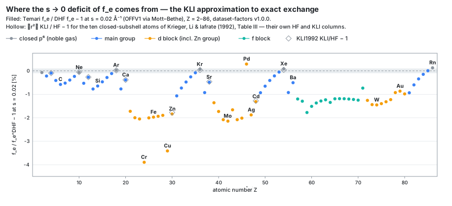
f_e / f_e^DHF − 1 at s = 0.02 for Z = 2–86, with the KLI/HF ratio of ⟨r²⟩ from Krieger et al. (1992) overlaid

Every noble gas sits at zero (He, Ne, Ar, Kr, Xe, Rn: −0.07 … +0.13 %), and so does Pd (4d¹⁰, no 5s: +0.3 %).
The dip is the d block: the 3d and 4d rows sit at −1.7 … −2.1 % (Sc–Ni, Zr–Rh; Y −1.4 %, Tc −1.7 %), the 5d row at −0.9 … −1.5 % (Hf–Hg), and the dip is deepest where a single 4s electron sits over a half-filled or filled 3d shell — Cr −3.9 %, Cu −3.4 %. The main group climbs back to zero across each period; the lanthanides sit at −1.2 … −1.8 %.
The hollow diamonds are not Temari's numbers at all. They are the ratio \(\langle r^2 \rangle_{\rm KLI}/\langle r^2 \rangle_{\rm HF} - 1\) read from Table III of Krieger et al. (1992), the paper that introduced the KLI approximation, for the ten closed-subshell atoms they tabulate. They fall on the filled dots to within 0.07 percentage points everywhere — Be, Ne, Mg, Ar, Ca, Zn, Kr, Sr, Cd, Xe — including the −1.8 % of Zn (the 0.07 case) and the −1.3 % of Cd. Temari's non-relativistic KLI reproduces the paper's KLI column to its four printed decimals for these atoms (selftest T20 gates Ne and Ar; Mg, Ca, Zn, Sr and Cd were checked the same way), so the agreement is between the approximation and its reference, not an accident of two errors.

The suspect is therefore identified: the deficit tracks the KLI approximation itself. For the ten closed-subshell atoms this is a direct match; for the open-shell d elements, where no published KLI-versus-HF \(\langle r^2 \rangle\) exists, it is an inference from the same pattern (a Dirac-plus-KLI against DHF comparison at finite \(s\) set beside a non-relativistic KLI-versus-HF one — the relativistic and \(s^2\) pieces evidently cancel to the 0.07-point level where both are available). In the same table the exchange-only optimized effective potential (OEP) agrees with Hartree–Fock to 0.1 % for every one of the ten atoms, Zn included, so what is missing is what KLI drops relative to OEP — the orbital-shift terms; that these bind a diffuse \(n\)s electron slightly too tightly over a compact \((n-1)\)d shell is the natural reading of the Zn/Cd/Cr/Cu pattern, not something separately proven here.

Take-away. The consequence for the shipped tables is measured and localized: \(f_x\) stays within 0.22 % of DHF for every d-block element (Sc 0.21 %, Cr 0.17 %, Fe 0.17 %, Cu 0.15 %, Au 0.07 %; worst points at \(s\) = 0.3–0.7 Å⁻¹, where the deficit is a small fraction of \(Z\)); \(f_e\) for \(s \ge 0.4\) Å⁻¹ sits within 0.16 % for the d block and within 0.14 % for every element from \(s \ge 0.5\); and \(f_e\) as \(s \to 0\) is low by up to 2 % for the d block and 4 % for Cr and Cu. Users of \(f_e(0)\) or of the mean inner potential for transition metals should know this; users of structure factors at ordinary \(s\) see at most the 0.16 % above.

3. Inner-shell ionization form factor F(s)¶

Dataset v5.0.0 (κ-resolved Dirac continuum, relaxed core-hole final state) against the two references that exist for this quantity: the tables of Oxley & Allen (2000) and the shape factors distributed with the µSTEM code (Allen et al., 2015). Both references share a Hartree–Slater atomic potential and a one-component (Schrödinger) continuum wave for the ejected electron.

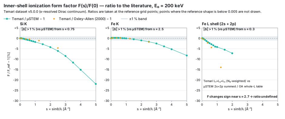
Making the three comparable took some care. The comparison is of the normalized shape \(F(s)/F(0)\) at \(E_0 = 200\) keV, taken at the reference grid points (Temari's 0.05 Å⁻¹ table is interpolated to them; the references are not interpolated). Oxley & Allen's L table is the whole L shell, so for the third panel the shipped L₁, L₂, L₃ rows are combined with their \(N_0\) weights and µSTEM's separate 2s and 2p factors are summed — the same Temari composite is then divided by each reference, which is what makes the two symbol sets comparable to each other. (The 2s : 2p weight is a by-product check: Temari's \(N_0(\mathrm{L_1}) / [N_0(\mathrm{L_2}) + N_0(\mathrm{L_3})]\) is 0.187 and µSTEM's \(F_{2s}(0)/F_{2p}(0)\) is 0.189.)

F(s)/F(0) of Si K, Fe K and the Fe L shell at 200 keV: ratio to µSTEM and to Oxley–Allen minus one

What the figure shows:

Agreement within 1 % holds up to \(s \approx 0.75\) Å⁻¹ for Si K, ≈ 2 for Fe K and ≈ 0.3 for the Fe L shell (against µSTEM), and beyond that Temari's shape falls faster than both references, monotonically: −22 % at \(s = 5\) for Si K, −8 % for Fe K, −7 % at \(s = 2\) for the Fe L shell. The picture at 100 and 300 keV is the same (the Si K curve crosses −1 % between \(s = 0.5\) and 0.75 at all three voltages). The lighter the element and the higher the shell, the earlier the departure — Fe K is the best case here, not the typical one. (For orientation: at Si K, \(s = 1\), the retired v3 tables with their scalar-relativistic continuum sat at −2.6 % against µSTEM, the older non-relativistic v2 at −1.5 %, v5 at −1.7 % — the κ-resolved Dirac continuum brought the shape back to within 0.2 points of the non-relativistic result, as the small size of the true relativistic effect requires.)
The two references also disagree with each other, more so for the L shell: with the same Temari composite in the numerator, Oxley–Allen's whole L gives −14 % at \(s = 1.25\) where µSTEM's 2s + 2p gives about −5 %, i.e. Oxley–Allen sits some 11 % above µSTEM there (1.6 % at \(s = 0.625\)). For K the two references agree with each other to 1.5 % (Si) and 0.1 % (Fe) up to \(s = 2.5\).
The L-shell ratio ends at \(s = 2\) because \(F\) changes sign near \(s \approx 2.7\) Å⁻¹ (the shipped \(F\) is signed — see Data); a ratio through a zero carries no information.

What this comparison cannot decide. Which side is closer to the truth at large \(s\) — no experimental comparison at that level is used here, and for the L shell the two references do not agree with each other there either (for K they agree with each other to 1.5 % up to \(s = 2.5\), so there Temari differs from two references that agree with each other — which still does not say which is right). What is known is how much it matters for the quantity the tables are used for: the propagation study found that STEM-EDX/ALCHEMI observables are sensitive to \(s < 2\) Å⁻¹ only, with \(s > 4\) contributing at the 10⁻⁹ level — for the one crystal and one orientation tested. The region where the curves part is, for those observables, the region that does not matter; the region that matters is where they agree.

What to take away¶

Quantity	What can be concluded	What should not be concluded
\(f_x\)	For the atoms shown, Temari follows exchange-only DHF to a fraction of a percent over 0–6 Å⁻¹ (under 0.1 % RMS below \(s = 2\)) — comparable to the standard fits over their own range, and computed over the whole 0–6 Å⁻¹ without a fit-range limit	That the atom is complete (no correlation, no bonding, no experiment enters)
\(f_e\)	Same at ordinary \(s\); a KLI-specific deficit of up to 2 % (4 % for Cr, Cu) at \(s \to 0\) for the d block, traced to the approximation itself	That every transition metal is off by one fixed percentage, or that the deficit reaches structure factors at ordinary \(s\)
\(F(s, E_0)\)	The shape agrees with the references within 1 % up to \(s \approx 0.75\) (Si K), 2 (Fe K) and 0.3 Å⁻¹ (Fe L shell), and falls faster beyond; the tested observables respond to \(s < 2\) only, where the departure reaches a few percent for Si K and the Fe L shell and 1 % for Fe K; the L-shell references disagree with each other by 11 %	That either side is right at large \(s\); that one crystal's propagation result covers every observable

Regenerating the figures¶

python tools/make_comparison_figures.py              # Si and Fe, E0 = 200 keV
python tools/make_comparison_figures.py --z 14,26,79 # more columns
python tools/make_comparison_figures.py --e0 300     # another E0 for F(s)

The script needs the references on the local disk (they are not in the repository — refs/README.md lists what goes where) and writes only ratios and deviations, to docs/src/assets/figures/. It prints the same deviations to the terminal, never a reference value. What the SVGs carry is the ratio, at roughly 10⁻⁴ percentage-point resolution — a derived comparison figure, which is where the contributing guidelines draw the line: deviations and ratios may be published, transcribed values may not.

References¶

Allen, L. J., D'Alfonso, A. J. & Findlay, S. D. (2015). Modelling the inelastic scattering of fast electrons. Ultramicroscopy 151, 11–22.
Cromer, D. T. & Mann, J. B. (1968). X-ray scattering factors computed from numerical Hartree–Fock wave functions. Acta Crystallographica A 24, 321–324.
Doyle, P. A. & Turner, P. S. (1968). Relativistic Hartree–Fock X-ray and electron scattering factors. Acta Crystallographica A 24, 390–397.
Kirkland, E. J. (2010). Advanced Computing in Electron Microscopy, 2nd ed. Springer, New York.
Krieger, J. B., Li, Y. & Iafrate, G. J. (1992). Construction and application of an accurate local spin-polarized Kohn–Sham potential with integer discontinuity: Exchange-only theory. Physical Review A 45, 101–126.
Olukayode, S., Froese Fischer, C. & Volkov, A. (2023). Revisited relativistic Dirac–Hartree–Fock X-ray scattering factors. I. Neutral atoms with Z = 2–118. Acta Crystallographica A 79, 59–79.
Oxley, M. P. & Allen, L. J. (2000). Atomic scattering factors for K-shell and L-shell ionization by fast electrons. Acta Crystallographica A 56, 470–490.
Peng, L.-M., Ren, G., Dudarev, S. L. & Whelan, M. J. (1996). Robust parameterization of elastic and absorptive electron atomic scattering factors. Acta Crystallographica A 52, 257–276.
Prince, E. (ed.) (2004). International Tables for Crystallography, Vol. C, 3rd ed. Kluwer, Dordrecht.
Waasmaier, D. & Kirfel, A. (1995). New analytical scattering-factor functions for free atoms and ions. Acta Crystallographica A 51, 416–431.