SAED (Selected Area Electron Diffraction) Simulation
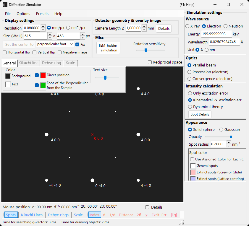
SAED (Selected Area Electron Diffraction) simulation calculates single-crystal electron diffraction patterns produced by a parallel electron beam. This is the default mode of the diffraction simulator.
This page lists every setting that appears in the Spot property panel on the right when you choose Wave Length = Electron and Incident beam mode = Parallel. For window-wide operations such as drawing and saving, see the overview page.
GUI conditions: Wave Length = Electron, Incident beam mode = Parallel, Intensity calculation = Only excitation error / Kinematical / Dynamical.
Overview
Simulates the diffraction pattern produced when a parallel electron beam passes through a thin specimen. Spot positions are fixed by the geometric relationship between the Ewald sphere and the reciprocal-lattice points, and the brightness of each spot is computed according to the selected intensity-calculation mode.
Wave Length
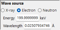
Set the radiation source to Electron. Enter the energy (keV) or wavelength (nm) and the relativistically corrected wavelength is computed. For X-ray and neutron sources, see X-ray diffraction simulation.
Incident beam mode
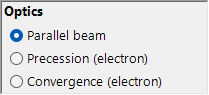
Set the incident-beam geometry to Parallel. This is the standard plane-wave geometry used for SAED and X-ray diffraction.
Note: For electrons you can choose Parallel / Precession (electron = PED) / Convergence (CBED). Choosing Precession gives a PED simulation and choosing Convergence gives a CBED simulation; in both cases the intensity calculation automatically switches to Dynamical.
Intensity calculation
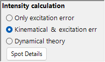
Selects how spot intensities are computed.
Only excitation error
Intensity is determined solely from the geometric distance between the Ewald sphere and the reciprocal-lattice point (the excitation error \(S_g\)). It is largest at \(S_g = 0\) — exactly on the sphere — and falls off as \(\lvert S_g\rvert\) grows, reaching zero once \(\lvert S_g\rvert\) exceeds the Radius given for the reciprocal-lattice point. Because the crystal structure factor is ignored, this is the fastest mode and is suited to checking diffraction-spot positions.
Kinematical
In addition to the excitation error, the kinematical structure factor \(\lvert F_{hkl} \rvert^2\) is folded into the intensity. Extinction rules are correctly reflected, making this mode suited to thin specimens or weak diffraction.
Dynamical (Bloch-wave method, electron only)
A rigorous dynamical calculation by the Bloch-wave method (Bethe method). It reproduces multiple scattering and the thickness-dependent variation of intensity, and is required for thick specimens or strong diffraction. Available only when Electron is selected. For the theory, see Appendix A3. Bloch-wave method.
Note: When Dynamical is selected, a Bloch wave settings panel appears below.
Bloch wave settings (Dynamical theory)
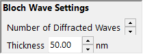
Active only when Intensity calculation = Dynamical.
| Parameter | Description |
|---|---|
| Number of diffracted waves | Number of Bloch waves included in the eigenvalue problem. Larger values give more accurate intensities but increase computation time as \(O(N^3)\) |
| Thickness | Specimen thickness (nm) used in the dynamical calculation |
Spot appearance
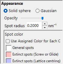
Controls how each diffraction spot is rendered.
- Solid sphere / Gaussian : the geometric model of the reciprocal-lattice point. Solid sphere draws the cross-section (a circle) between a sphere of radius \(R\) and the Ewald sphere, with the circle area corresponding to the diffraction intensity; Gaussian draws the cross-section (a 2-D Gaussian) of a 3-D Gaussian with \(\sigma = R\), with its integral corresponding to the diffraction intensity.
- Opacity : transparency of the spot (0 = transparent, 1 = opaque).
- Radius (R) : virtual radius of the reciprocal-lattice point. The spot size is fixed by the combination of Appearance mode and Intensity calculation (e.g. Solid sphere + Dynamical gives a radius proportional to \(I_\text{dyn}^{1/2}\)).
- Brightness : active only in Gaussian mode. Integrated intensity of the rendered Gaussian.
- Color scale : Gray scale or Cold-warm.
- Log scale : display intensities on a logarithmic scale. Useful for patterns with large intensity contrast.
- Spot color : spot colour used when the colour scale is not in use.
- Color per crystal : when checked, spots are drawn in the colour assigned to each crystal.
Spot labels
The labels overlaid on the spots are selected from the toolbar.
| Label | Content |
|---|---|
| Index | Miller indices \((hkl)\) |
| d | interplanar spacing \(d\) |
| 1/d | reciprocal of the interplanar spacing \(1/d\) |
| Distance | spot-to-spot distance on the detector |
| 2θ | scattering angle \(2\theta\) (same definition as the concentric 2θ scale circles) |
| χ | azimuth angle \(\chi\), measured from the upward (12 o'clock) direction, positive clockwise (same definition as the radial azimuth scale lines) |
| Excit. Err. | excitation error \(S_g\) |
| |Fg| | absolute value of the structure factor \(\lvert F_{hkl} \rvert\) |
Shared operations
Detector information, flipping, reciprocal-space display, Kikuchi lines, Debye rings, scale lines, colour settings, saving, and the like are common to all modes. See the overview page. The per-reflection details obtained from the dynamical calculation can be browsed in diffraction spot information.