EBSD Simulation¶

EBSD Simulator simulates the electron backscatter diffraction (EBSD) patterns — Kikuchi patterns — obtained in a scanning electron microscope (SEM), using dynamical-theory calculations. It computes the angular/energy/depth distribution of backscattered electrons (BSE) by a Monte-Carlo simulation, builds a dynamical (Bloch-wave) master pattern of the crystal, and projects it onto the detector for the current crystal orientation. An experimental EBSD image can also be loaded and indexed: the orientation that best explains it is searched for automatically (Experimental image).

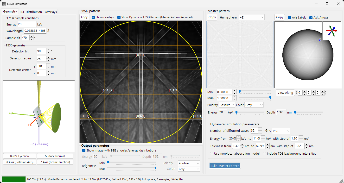
The window has three columns.

Left : simulation conditions. The tabs select Geometry (sample/detector geometry and a 3D view), BSE Distribution (backscattered-electron distributions), and Overlays (Kikuchi lines and other annotations).
Centre : the EBSD (Kikuchi) pattern for the current crystal orientation. Below it, the tabs select Output parameters of dynamical EBSD pattern and Experimental image.
Right : the orientation-independent master pattern, in the 2D and 3D tabs.

The status bar at the bottom shows the progress of the running calculation and a summary of its result.

Keyboard & mouse shortcuts¶

The centre EBSD (Kikuchi) pattern and the right-hand master-pattern views respond to different mouse actions.

Shortcut	Action
`F1`	Open this page of the online manual
Left-drag the pattern near the centre	Tilt the crystal
Left-drag the pattern's outer area	Spin the crystal
Double-click the pattern	Pick the detector sub-cell under the cursor and show its statistics
Drop an image file on the window	Load it as the experimental EBSD image
Left-drag a 3-D view (geometry / master sphere)	Rotate it
Right-drag, or Mouse wheel, on a 3-D view	Zoom
`CTRL` + Right double-click a 3-D view	Toggle orthographic / perspective
Drag / wheel on the 2-D master pattern	Pan / zoom the image

The 3-D views use ReciPro's standard view navigation (panning disabled).

→ See 21. Keyboard & mouse shortcuts for every window at a glance.

Workflow¶

Pressing Build Master Pattern runs the following steps in order.

Monte-Carlo BSE simulation : using the current crystal composition, density, accelerating voltage and sample tilt, about 2.5 million electrons are tracked inside the sample (elastic scattering: Mott/NIST cross-sections; inelastic scattering: dielectric-response model). This yields the joint distribution of penetration depth × exit direction × exit energy of the backscattered electrons.
Automatic range selection : from that distribution, the energy range (from the incident energy down to about the 80th percentile of energy loss) and depth range (to about the 99th percentile of penetration depth) used in the dynamical calculation are set automatically.
Master-pattern build : for each energy and depth, the dynamical diffraction (Bloch-wave) problem is solved and integrated over the sphere of directions, weighted by the Monte-Carlo distribution, to give the backscatter diffraction intensity in every direction. The result is stored on an equal-area (Rosca–Lambert) grid.
Projection onto the detector, with weighting : for the current crystal orientation, the intensity for the direction subtended by each detector pixel is looked up in the master pattern and drawn as the Kikuchi pattern, optionally weighted by the BSE angular/energy distribution.

The energy and depth ranges are set automatically in steps 1–2, but can be adjusted manually before building.

Geometry¶

SEM & sample conditions¶

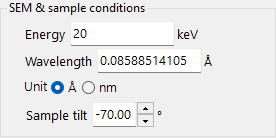
Energy : accelerating voltage of the incident beam (keV).
Wavelength : electron wavelength, linked to Energy. Unit selects Å or nm.
Sample tilt : sample tilt angle (typically −70°). The large tilt in EBSD increases the backscattered-electron yield.

EBSD geometry¶

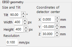
The detector (phosphor screen) is a rectangle defined by a pixel count and a pixel size.

Size and Tilt : Tilt is the tilt of the detector plane (°); Width and Height are the number of detector pixels.
Resolution : the physical size of one detector pixel (mm/px). The physical detector size is therefore Width × Resolution by Height × Resolution.
Coordinates of detector center : position X, Y, Z of the detector centre relative to the beam-impact point (mm). Y and Z, together with the tilt, determine the camera length; X is the left–right offset.

Loading an experimental image sets Width and Height to the image size, so that one detector pixel corresponds to one image pixel (Resolution is left unchanged).

The geometry can be inspected in the 3D view on the Geometry tab.

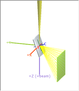
The grey plate is the sample, the green rectangular slab is the detector, and the purple +Z (=beam) is the incident beam. The crystal a / b / c axes (fixed to the sample) are also shown. The buttons Bird's-Eye View, Surface Normal, X Axis (Rotation Axis) and Z Axis (Beam Direction) snap the view to standard directions. See Appendix A1. Coordinate Systems for the coordinate-system definitions.

BSE Distribution¶

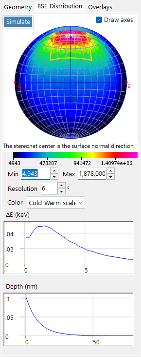
The BSE Distribution tab shows the Monte-Carlo backscattered-electron distributions. Use Simulate to recompute them.

Stereonet : angular distribution (histogram of exit directions) of the backscattered electrons. The centre is the surface-normal direction, and the yellow outline marks the rectangular region subtended by the detector. Draw axes overlays the crystal axes, and the colour scale (Min / Max, Resolution, Color) is adjustable.
ΔE (keV) : energy-loss distribution of the backscattered electrons.
Depth (nm) : distribution of the depth at which the detected backscattered electrons had their last inelastic scattering event — the same depth definition that weights the master pattern.

These distributions are computed by the same Monte-Carlo engine as Electron trajectory and are used to weight the master pattern.

Overlays¶

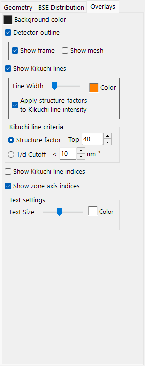
The Overlays tab configures the annotations drawn on the EBSD pattern.

Background color : background colour.
Detector outline : the detector outline. Show frame (the yellow rectangle at the detector edge) / Show mesh (division grid).
Show Kikuchi lines : draw Kikuchi lines. Line Width / Color, and Apply structure factors to Kikuchi line intensity (each line fades toward the background in proportion to its structure factor).
Kikuchi line criteria : which Kikuchi lines to draw: Structure factor (Top N by structure factor) or 1/d Cutoff (those with 1/d below a threshold, nm⁻¹).
Show Kikuchi line indices : show indices of the Kikuchi lines (bands).
Show zone axis indices : show zone-axis indices.
Text settings : Text Size / Color of the index labels.

Master pattern¶

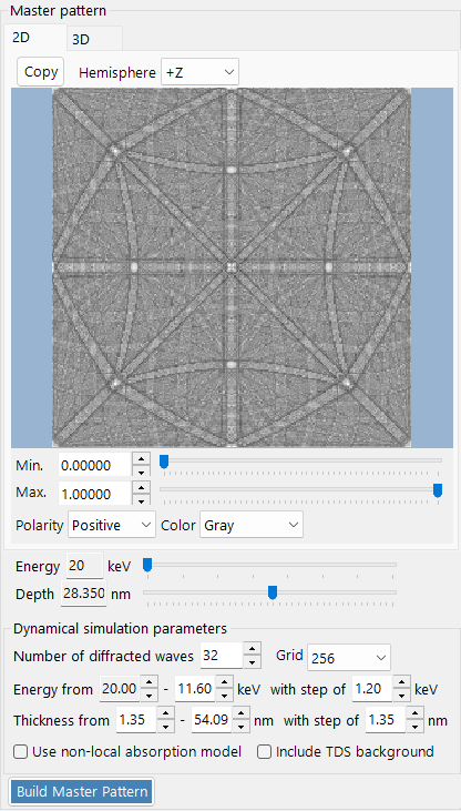
The master pattern is the backscatter diffraction intensity over all directions, computed in advance by the dynamical theory with Build Master Pattern (Stop interrupts the running calculation).

2D tab : equal-area (Lambert) projection of a hemisphere. Hemisphere selects the projected hemisphere (+Z / −Z).
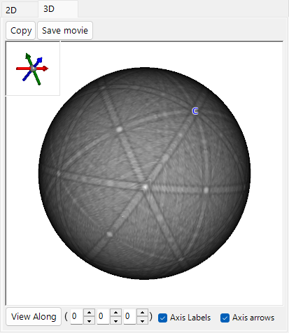
3D tab : a sphere with the intensity mapped onto it. It can be rotated with the mouse, and an inset at the top-right shows the synchronised crystal axes (a/b/c). Axis Labels / Axis arrows toggle the labels/arrows, and View Along looks down the zone axis [u v w] entered next to it.
Energy / Depth sliders : select the energy/depth slice to preview.
Either view can be sent to the clipboard with Copy.

Dynamical simulation parameters¶

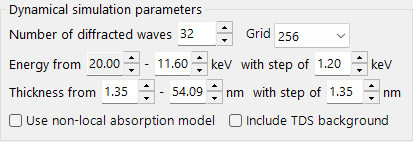
Number of diffracted waves : number of diffracted beams (waves) included in the Bloch-wave calculation. More waves are more accurate but slower.
Grid : resolution of the master-pattern grid (default 256).
Energy from … to … with step of … : energy range and step integrated over (keV); set automatically from the Monte-Carlo result.
Thickness from … to … with step of … : depth range and step integrated over (nm); likewise set automatically.
Use non-local absorption model : use the non-local absorption form.
Include TDS background : include the thermal-diffuse-scattering (TDS) background.

EBSD pattern¶

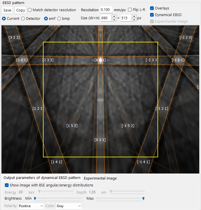
The centre panel shows the EBSD (Kikuchi-band) pattern for the current crystal orientation. The bar above the pattern controls what is drawn and how it is copied.

Dynamical EBSD : projects the built master pattern onto the detector; unchecked leaves a plain background.
Overlays : draws the Kikuchi lines, indices and detector outline configured in the Overlays tab.
Experimental image : overlays the loaded experimental image (see below).
Flip L-R : mirrors the pattern and all its overlays left-right. Unchecked (the default) is the view from the detector towards the sample, i.e. the pattern as an EBSD camera records it; check it only if your experimental image has the opposite handedness.
Resolution (mm/px) and Size (W×H) (px) : resolution and size of the displayed view.
Copy : copies the pattern to the clipboard, using the range and format selected next to it.
Current copies the area currently shown (as panned and zoomed); Detector copies only the detector area, in which case the yellow frame is left out so the image ends exactly at the detector edge.
emf copies an Enhanced Metafile, keeping the Kikuchi lines and index labels as vectors; bmp rasterizes everything.
Match detector resolution copies at one image pixel per detector pixel (the longer side is clamped to 4096 px). Unchecked, the on-screen resolution is used.

Output parameters of dynamical EBSD pattern¶

Show image with BSE angular/energy distributions : when checked, the pattern is composited by weighting with the BSE distribution (energy, depth, direction) rather than a single slice.
Energy / Depth : when the above is off, select the energy/depth slice to display.
Brightness (Min / Max), Polarity, Color : brightness range, polarity, and colour scale.

Experimental image¶

Drop an EBSD image file (TIFF, PNG, BMP or JPEG; 16-bit TIFF is read at full depth) anywhere on the window to load it as the experimental pattern. It is drawn over the detector area — above the simulated pattern and below the Kikuchi-line overlays — so the simulation can be compared with the measurement directly. Loading an image also sets the detector Width and Height to the image size.

Brightness (Min / Max) : black and white points of the overlaid image, as a fraction of its own intensity range (logarithmic sliders). These act on the experimental image only, not on the simulated pattern.
Opacity : opacity of the overlaid image, from 0 (invisible) to 100 % (opaque). Lower it to see the simulated pattern underneath.

The orientation that explains the image is then searched for with one of two engines.

Radon search : matches kinematical Kikuchi-band templates against the Radon (line-detection) map of the experimental image. It works without a master pattern; when one exists, the candidates are re-ranked by a robust ZNCC (zero-mean normalized cross-correlation) against the simulated pattern.
Dictionary search : generates dictionary patterns from the dynamical master pattern over all orientations and compares them all by robust ZNCC. It requires the master pattern and takes a few seconds, but is more reliable than Radon search.

Find orientation candidates runs the selected engine and lists up to 10 candidates, best first; when a master pattern is available the top candidate is refined to ±0.25°. The columns are:

Column	Meaning
#	Rank (0 = best)
Score	Radon band-evidence z value
Bands	Matched bands / predicted bands in the field of view
ZNCC	Correlation with the simulated pattern
Strong bands (hkl)	Indices of the matched bands (Radon search only)

Clicking a row applies that orientation to the whole program, so the simulated pattern is redrawn on top of the experimental one and the crystal orientation of every other window follows.

Calibrate geometry refines the detector geometry — pattern centre (PC) and detector distance (DD) — alternately with the orientation, by maximizing the ZNCC between the simulated and experimental patterns. It requires the master pattern, keeps the detector tilt fixed, and writes the result back to the Coordinates of detector center X/Y/Z boxes. Since the beam scan of an SEM moves the pattern centre by only a fraction of a millimetre, one calibration at the beginning of an experiment is usually enough for a whole series of images.