HRTEM / STEM Simulator¶

The HRTEM/STEM Simulator simulates TEM lattice-fringe (HRTEM) images, STEM images, and projected crystal potentials for the selected crystal and orientation. Click Simulate to run.

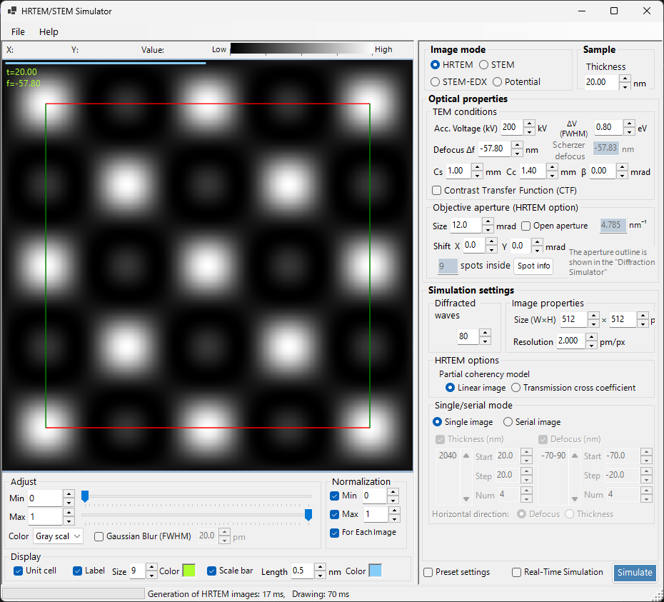
The window is split into two halves. The left side displays the simulation result and controls its appearance (image panes, brightness, color, scale bar, and so on); the right side holds the calculation conditions (Optical properties and Simulation settings).

This page and the mode pages¶

This page (overview): the operations common to every mode, together with the result display and adjustment controls on the left side.
Mode pages: every setting that appears on the right side for that mode, covered so that each page is self-contained (some settings therefore appear on more than one page).

Mode	Contents	Page
HRTEM	High-resolution TEM lattice-fringe images	HRTEM simulation
STEM	Scanning transmission electron microscope images (BF / ABF / LAADF / HAADF)	STEM simulation
Potential	Projected crystal potential (\(U_g\) / \(U'_g\))	Potential simulation

Keyboard & mouse shortcuts¶

Results are shown as one or more image panes. They use ReciPro's standard image-view navigation, and all panes pan and zoom together.

Shortcut	Action
`F1`	Open this page of the online manual
`CTRL`+`C` (image grid focused)	Copy the image(s) to the clipboard as a metafile
Left-drag / Middle-drag	Pan the image (all panes move together)
Mouse wheel up / down	Zoom in (×2) / out (×0.5) at the cursor
Right-drag a box	Zoom in to the selected region
Right-click / Right double-click	Zoom out (×0.5)
`CTRL` + Right-drag a box	Select a rectangular area
Left double-click a pane	Maximize that pane / restore the grid (multi-pane layouts)
Move the mouse (no button)	Read the position (pm) and pixel value at the cursor

→ See 21. Keyboard & mouse shortcuts for every window at a glance.

Quick routes by goal¶

Goal	Start from	Reference
Calculate one HRTEM image	Set Image mode to HRTEM, then set the accelerating voltage and defocus in TEM conditions	HRTEM simulation, HRTEM image formation
Calculate a STEM image	Set Image mode to STEM, then set the convergence angle and detector in STEM options	STEM simulation, STEM calculation
View the projected potential	Set Image mode to Potential	Potential simulation
Generate a thickness / defocus series	In HRTEM, configure Single/serial mode and the image conditions	HRTEM simulation
Use HAADF-STEM with TDS	Set non-zero atomic temperature factors and move the STEM detector to LAADF / HAADF	STEM calculation

Basic workflow¶

Select the crystal and orientation in the main window, then open this window.
Choose HRTEM, STEM, or Potential in Image mode.
Set the accelerating voltage, defocus, aberrations, aperture, STEM convergence angle, and so on in Optical properties (see the mode pages).
Set the thickness, image size, resolution, Bloch-wave count, partial-coherence model, and so on in Simulation settings (see the mode pages).
Click Simulate, then tune the appearance with Adjust, Normalization, and Display on the left as needed.

Selecting the image mode¶

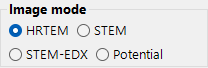
Image mode at the top right selects the kind of calculation. The panels on the right (Optical properties and Simulation settings) change to match the mode you choose.

HRTEM — high-resolution TEM lattice-fringe images → HRTEM simulation
STEM — scanning transmission electron microscope images → STEM simulation
Potential — projected crystal potential → Potential simulation

Image area (left side)¶

The left half of the window shows the simulated image. The status bar across the top reports the cursor position (X:, Y:) and the image Value: (intensity) under the cursor, next to a Low → High intensity scale that reflects the current color map and brightness range.

When several images are produced (a serial image, or the magnitude/phase of a potential) they are tiled in a grid, and all panes zoom and pan together.

Displaying and adjusting results (left panel)¶

The panel at the lower left adjusts how the result looks — brightness, color, normalization, and overlays. These apply to every mode and take effect without recalculating.

Adjust¶

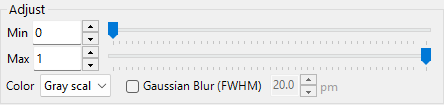
Min / Max : lower (black) and upper (white) ends of the displayed intensity range. Use the trackbars to adjust the contrast.
Color : color scale of the image — Gray scale or Cold-Warm (blue to red).
Gaussian Blur (FWHM) : when checked, applies a Gaussian blur with the full width at half maximum (pm) given on the right, approximating a finite resolution (point-spread function).

Normalization¶

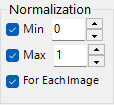
For Each Image : when checked, normalizes each image separately (when unchecked, the whole series shares a common scale).
Min / Max : fixes the lower / upper end of the normalization to the value given on the right instead of the minimum / maximum of the image.

STEM image¶

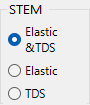
Shown in STEM mode only. Selects which scattering component of the calculated STEM image is displayed (Elastic, TDS, or Elastic & TDS). Because it is specific to STEM, it is also described on the STEM simulation page.

Display¶

Sets the items overlaid on the image.

Unit cell : overlays the outline of the projected unit cell, so you can relate the image contrast to the crystal lattice.
Label : overlays labels such as thickness, defocus, and indices. Size (font size) and Color can be specified.
Scale bar : overlays a scale bar. Length (nm) and Color can be specified.

Running the simulation¶

Simulate : runs the calculation with the current crystal, microscope conditions, thickness, defocus, and display settings.
Stop : aborts the running calculation (shown only while calculating).
Real-Time Simulation : when checked, recalculates immediately as the crystal is rotated (hidden in STEM mode).
Preset settings : toggles the preset window, which stores and recalls TEM imaging conditions.

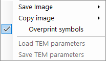
Save Image : save as as Image (PNG format), as Image (TIFF format), or as Metafile (EMF). Save individually for serial image mode writes the images of a serial run one by one.
Copy image : copy to the clipboard as Image or as Metafile (EMF).
Overprint symbols : burns the unit cell, labels, and scale bar into the saved image.
Load TEM parameters / Save TEM parameters : save the optical conditions (accelerating voltage, aberrations, and so on) to a file and restore them.

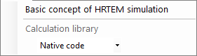
Basic concept of HRTEM simulation : opens the explanation of HRTEM image formation (Appendix A3.2).
Calculation library : selects the calculation library — Native code (fast C++/Eigen) or Managed code (.NET). Native is normally faster.