Atomic Scattering Factors¶

The atomic scattering factor (or form factor) measures how strongly a single atom scatters the incident beam as a function of the scattering variable \(s=\sin\theta/\lambda\). The three radiations interact with completely different parts of the atom, so their scattering factors have different magnitudes, units, and angular dependence. This is the single most important reason the Scattering factors tab looks so different between X-ray, electron, and neutron beams.

X-rayElectronNeutron

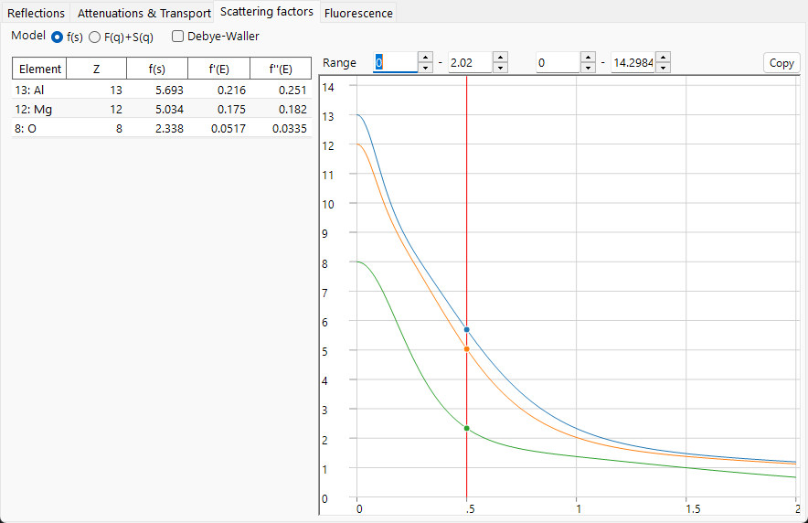
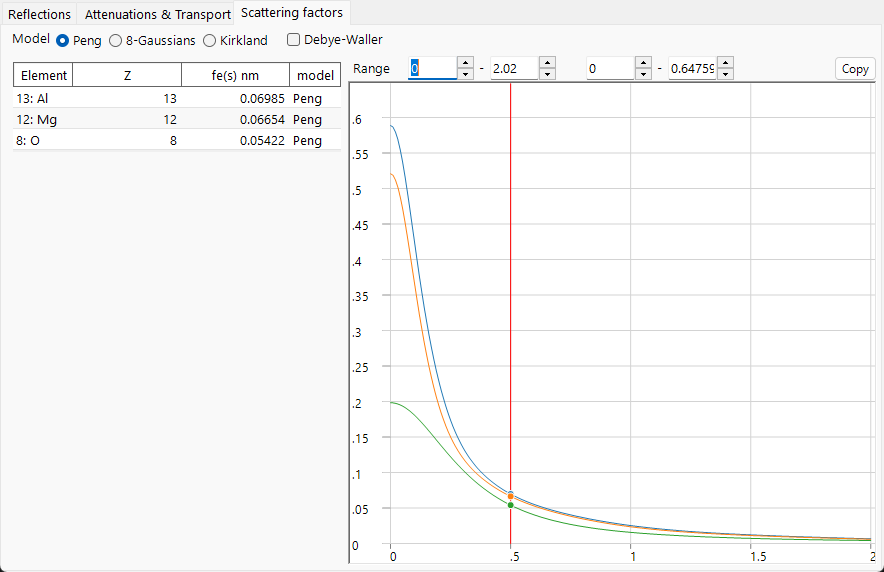
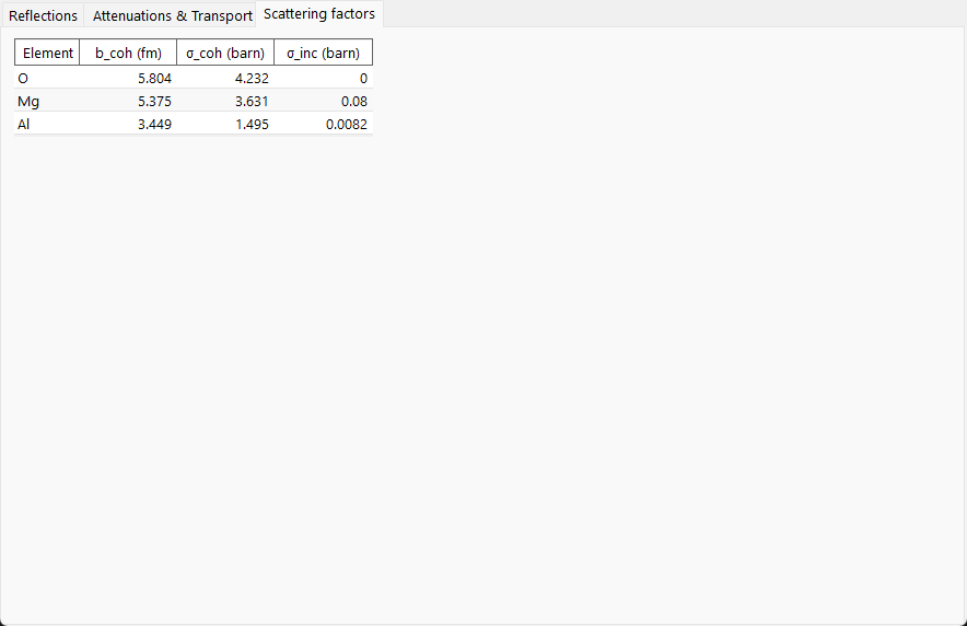
X-rays — scattering by the electron cloud¶

X-rays are scattered by the electrons of the atom. A single free electron scatters with the classical Thomson differential cross section, set by the classical electron radius \(r_e = e^2/(4\pi\varepsilon_0 m_e c^2) \approx 2.82\times10^{-5}\ \text{Å}\):

\[\left(\frac{d\sigma}{d\Omega}\right)_e = r_e^2\,\frac{1+\cos^2 2\theta}{2}.\]

The atom's electrons are distributed in space with number density \(\rho_e(\mathbf r)\), and the atomic scattering factor is the Fourier transform of that density. The atomic cross section is then the single-electron cross section scaled by \(|f_0|^2\):

\[f_0(\mathbf Q) = \int \rho_e(\mathbf r)\, e^{\,i\mathbf Q\cdot\mathbf r}\, d^3r , \qquad \left(\frac{d\sigma}{d\Omega}\right)_\text{atom} = r_e^2\,\frac{1+\cos^2 2\theta}{2}\,|f_0(s)|^2 .\]

In the forward direction (\(s\to 0\)) every electron scatters in phase, so \(f_0(0) = Z\), the atomic number. The factor is expressed in electron units (multiples of the Thomson amplitude — the second equation above makes this explicit).
As \(s\) increases, scattering from different parts of the cloud goes out of phase and \(f_0(s)\) falls off. A diffuse (outer, valence) electron distribution makes \(f_0\) drop quickly; tightly bound core electrons keep contributing to high \(s\).

In practice \(f_0(s)\) is tabulated as a sum of Gaussians (the Waasmaier–Kirfel analytical form that ReciPro uses, an extension of the older Cromer–Mann tables),

\[f_0(s) = \sum_{i} a_i\, e^{-b_i s^2} + c ,\]

which is what ReciPro evaluates for the curve. The coefficients are tabulated for \(s\) in Å⁻¹, so each \(b_i\) has units of Å²; ReciPro carries \(s^2\) internally in nm⁻² and applies the factor-100 conversion noted in the index.

Anomalous (resonant) dispersion¶

The Fourier-transform picture assumes the electrons scatter as if free. When the photon energy approaches an absorption edge, the bound electrons respond resonantly and two energy-dependent correction terms appear:

\[f(s,E) = f_0(s) + f'(E) + i\,f''(E) \qquad \text{(textbook, } e^{+i\phi}\ \text{convention).}\]

\(f'(E)\) : real dispersion correction (reduces the effective electron count near an edge).
\(f''(E)\) : imaginary part, largest just above an edge.
The two are linked by the Kramers–Kronig relations, so a peak in absorption (\(f''\)) is accompanied by a dispersive swing in \(f'\).

These are not free parameters. Causality (Kramers–Kronig) ties \(f'\) to \(f''\), and the optical theorem ties \(f''\) directly to the photoabsorption cross section:

\[f'(E) = \frac{2}{\pi}\,\mathcal{P}\!\!\int_0^\infty \frac{E'\,f''(E')}{E'^2 - E^2}\,dE', \qquad f''(E) = \frac{\sigma_\text{abs}(E)}{2\,r_e\,\lambda}.\]

Here \(\sigma_\text{abs}\) is essentially the photoabsorption part of the attenuation (not the Rayleigh/Compton terms) — the same edge structure seen on the Attenuation & transport page.

ReciPro evaluates \(f'\) and \(f''\) at the current energy with the bundled xraylib library and lists them in the table (with \(f'' > 0\)). Two sign points matter. First, xraylib returns \(F_{ii}\) with the opposite sign to the crystallographic convention, so ReciPro negates it to report a positive \(f''\). Second, under ReciPro's \(\exp(-2\pi i\,\mathbf g\cdot\mathbf r)\) phase convention the complex factor that actually enters the structure factor is \(f_0 + f' - i f''\) — the \(+i f''\) written above belongs to the opposite (\(e^{+2\pi i}\)) convention. This is why F_inv (the imaginary part of the structure factor) becomes non-zero near an edge — see Structure factor.

Electrons — scattering by the electrostatic potential¶

A fast electron is charged, so it is scattered by the electrostatic potential \(V(\mathbf r)\) of the atom — the combination of the positive nucleus and the negative electron cloud. The electron scattering factor \(f_e\) is therefore the Fourier transform of the potential, which by Poisson's equation links it to the X-ray factor. The result is the Mott–Bethe relation:

\[f_e(s) = C_\text{MB}\,\frac{Z - f_0(s)}{s^2} \;\;\propto\; \frac{Z - f_X(Q)}{Q^2}.\]

The prefactor \(C_\text{MB}\) is built from fundamental constants and depends on the unit system and on whether \(s\) or \(Q\) is used. ReciPro does not evaluate this relation directly — it uses the fitted Peng / Kirkland / 8-Gaussian forms below — so it is given here for physical insight rather than computation. Written out with the constants (for \(s\) and \(f_e\) in Å),

\[f_e(s)\,[\text{Å}] = \frac{m_e e^2}{8\pi\varepsilon_0 h^2}\,\frac{Z - f_0(s)}{s^2} \simeq 0.023934\,\frac{Z - f_0(s)}{s^2}, \qquad s\ \text{in Å}^{-1},\]

with a further \(\times 0.1\) when ReciPro reports \(f_e\) in nm, and an extra relativistic \(\gamma\) factor (below) in the dynamical potential.

The physics is in the numerator \(Z - f_0\): the electron sees the difference between the nuclear charge \(Z\) and the screening electron cloud \(f_0\), i.e. the net atomic potential.

Magnitude. Because of the \(1/s^2\) factor, \(f_e\) is sharply peaked toward small angles and is far larger (in its own units) and more forward-directed than \(f_0\). This is why electron diffraction is dominated by low-order reflections and why dynamical (multiple) scattering matters — see Appendix A3.
Small-angle limit. For a neutral atom both \(Z-f_0\to 0\) and \(s^2\to 0\), so \(f_e(0)\) is finite (a \(0/0\) limit set by the mean-square atomic radius). For an ion the cloud no longer cancels \(Z\) and the long-range Coulomb tail makes \(f_e\) diverge as \(s\to 0\); tabulated ionic electron factors must be treated with care at the smallest angles.
Relativistic correction. At TEM energies the electron mass and wavelength are relativistic. The wavelength uses the relativistic form \(\lambda = h/\sqrt{2 m_0 e U\,(1 + e U/2 m_0 c^2)}\), and the interaction potential carries the relativistic factor \(\gamma = 1 + eU/m_0c^2\). ReciPro applies this correction when forming the dynamical potential.

ReciPro offers three parametrisations of \(f_e(s)\):

Peng : a five-Gaussian fit, \(f_e(s)=\sum_i a_i e^{-b_i s^2}\), convenient and widely used for elastic electron scattering.
Kirkland : a mixed Lorentzian + Gaussian fit, \(f_e(q)=\sum_i \dfrac{a_i}{q^2+b_i} + \sum_i c_i\,e^{-d_i q^2}\). Its independent variable is \(q = 2s = 1/d\), not \(s\) — a frequent source of factor-of-two errors when comparing models (\(q\) in Å⁻¹, with the fitted coefficients \(a_i,b_i,c_i,d_i\) in the corresponding units).
8-Gaussians : an eight-term fit valid over a wider \(s\) range.

Choosing one. All three fit the same underlying \(f_e(s)\) and agree closely at low \(s\); they differ mainly in range and in how the atomic core is represented. Peng (neutral atoms and common ions, accurate to \(s\approx2\text{–}6\) Å⁻¹) is the usual default for SAED/CBED structure factors; Kirkland extends to higher \(s\) with a Lorentzian core term, suited to HRTEM/STEM (recall \(q=2s\)); 8-Gaussians is for reflections reaching very high \(s\). For a light element the three are nearly indistinguishable; the differences show up for heavy elements at high angle.

Neutrons — scattering by the nucleus¶

Thermal neutrons are uncharged and interact with matter mainly through the strong nuclear force, whose range (femtometres) is utterly negligible compared with the neutron wavelength (ångströms). The interaction is represented by the Fermi pseudopotential, a point source whose strength is the scattering length \(b\):

\[V(\mathbf r) = \frac{2\pi\hbar^2}{m_n}\,b\,\delta(\mathbf r) \qquad\Longrightarrow\qquad \frac{d\sigma}{d\Omega} = |b|^2 .\]

Because the scatterer is point-like, \(b\) is independent of \(s\) — there is no form-factor fall-off, which is why the Scattering factors tab draws no curve for neutrons and shows a table of scattering lengths instead.

\(b\) is a property of the nuclide, not the electron configuration. It varies irregularly from element to element (and between isotopes), can be negative (e.g. ¹H, Ti, Mn), and bears no monotonic relation to \(Z\). This is the basis of neutron contrast (light atoms near heavy ones, isotope labelling).
Coherent vs incoherent. A real element is a mixture of isotopes and nuclear-spin states with different \(b\). Splitting \(b = \langle b\rangle + \delta b\) gives a coherent part (from the mean) and an incoherent part (from the spread):

\[\sigma_\text{coh} = 4\pi\,|\langle b\rangle|^2, \qquad \sigma_\text{inc} = 4\pi\big(\langle |b|^2\rangle - |\langle b\rangle|^2\big), \qquad \sigma_s = \sigma_\text{coh} + \sigma_\text{inc}.\]

The coherent part produces Bragg diffraction (it is what enters the structure factor); the incoherent part is a flat, isotropic background (large for ¹H, the reason for deuteration).

Tabulated values

ReciPro reads \(b_\text{coh}\) and the cross sections from a nuclide table rather than computing them. For resonant nuclides the listed \(\sigma_\text{coh}\) need not equal the naive \(4\pi b^2\), so the table values are authoritative. Magnetic neutron scattering (from unpaired electron spins, which does have an \(s\)-dependent form factor) is not modelled here.

At a glance¶

	X-ray	Electron	Neutron
Scattered by	electron cloud \(\rho_e(\mathbf r)\)	electrostatic potential \(V(\mathbf r)\)	nucleus (point)
\(s\) dependence	falls off (FT of cloud)	\(\propto (Z-f_0)/s^2\), strongly forward	none (\(b\) constant)
Forward value	\(f_0(0)=Z\)	finite (neutral) / divergent (ion)	\(b\)
Energy dependence	\(f',f''\) near edges	relativistic \(\lambda,\gamma\)	\(\sigma_\text{abs}\propto 1/v\) (not \(b\))
Typical magnitude order	\(\propto Z\)	forward-peaked, grows with \(Z\)	irregular, can be \(<0\)