Appendix A2. Dynamical Diffraction by the Bloch-Wave Method¶

This appendix gives an overview of the dynamical electron-diffraction theory used by ReciPro's Crystal Diffraction, CBED, and HRTEM/STEM simulators. ReciPro follows the Bethe / Bloch-wave formulation. The step-by-step calculation (optical potential, transmission coefficients, intensities) is described in Dynamical calculation (common core).

The wave equation in a crystal¶

A fast electron travelling through the periodic electrostatic potential of a crystal obeys the (high-energy, stationary) Schrödinger equation, which can be written as

\[\nabla^2 \Psi(\mathbf{r}) + 4\pi^2\left\{\, k_{vac}^2 + \sum_{\mathbf g} U_{\mathbf g}\, e^{2\pi i\,\mathbf g\cdot\mathbf r} \right\}\Psi(\mathbf{r}) = 0\]

\(k_{vac}\) : wavenumber of the electron in vacuum.
\(U_{\mathbf g}\) : Fourier component of the crystal potential for the reciprocal-lattice vector \(\mathbf g\). Because the potential is lattice-periodic, it is written as a Fourier series over the reciprocal lattice.

Bloch's theorem¶

Since the potential has the periodicity of the crystal lattice, the solutions are Bloch waves:

\[\Psi(\mathbf{r}) = b\!\left(\mathbf{k}^{(j)}, \mathbf{r}\right) = u(\mathbf{r})\exp\!\left(2\pi i\,\mathbf{k}^{(j)}\cdot\mathbf{r}\right)\]

\(u(\mathbf r)\) : a function with the same periodicity as the crystal lattice, so it can itself be expanded over the reciprocal lattice, \(u(\mathbf r)=\sum_{\mathbf g} C_{\mathbf g}^{(j)}\exp(2\pi i\,\mathbf g\cdot\mathbf r)\).
\(\mathbf{k}^{(j)}\) : the \(j\)-th Bloch wavevector.
\(C_{\mathbf g}^{(j)}\) : the amplitude (eigenvector component) of beam \(\mathbf g\) in the \(j\)-th Bloch wave.

Bethe's dynamical equation¶

Substituting the Bloch-wave expansion into the wave equation yields Bethe's dynamical equation — one coupled equation for each beam \(\mathbf g\):

\[\left[\,k^2 - \left(\mathbf{k}^{(j)} + \mathbf{g}\right)^2 + i\,U'_{g,g}\right]C_{\mathbf g}^{(j)} + \sum_{h \neq g}\left(U^C_{g-h} + i\,U'_{g,h}\right)C_{\mathbf h}^{(j)} = 0\]

\(U^C_{\mathbf g}\) : crystal potential for elastic scattering.
\(U'_{\mathbf g}\) : imaginary (absorption) potential, which accounts for thermal diffuse scattering (TDS). How it and the Debye–Waller factor enter is detailed in the calculation core.

Geometric definitions (Ewald sphere)¶

The vectors and scalars appearing above are defined on the Ewald sphere:

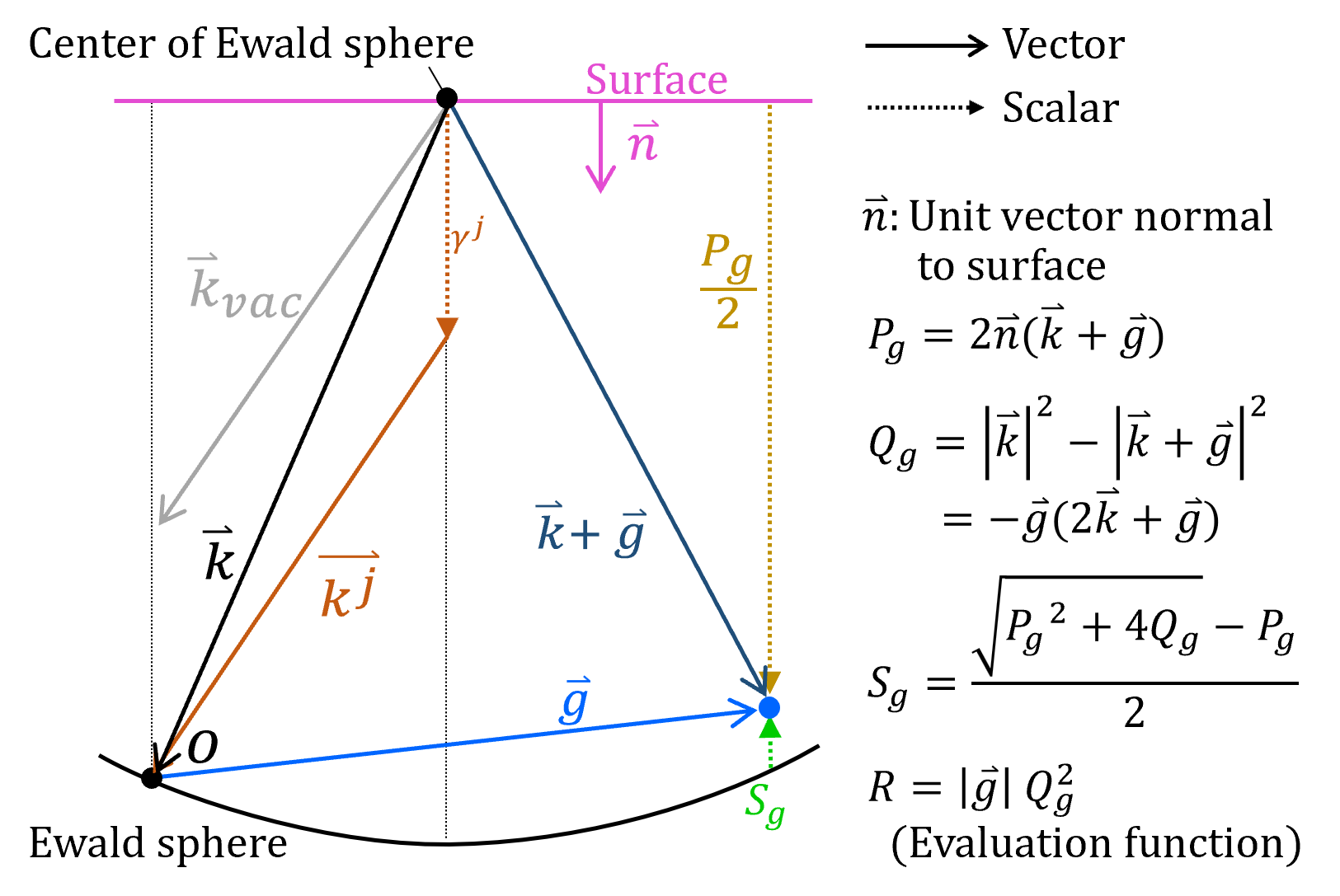
\(\hat{\mathbf n}\) : unit vector normal to the crystal surface.
\(\mathbf k\) : incident wavevector (its tip lies on the Ewald sphere); \(\mathbf k_{vac}\) is the vacuum wavevector.
\(\mathbf g\) : reciprocal-lattice vector; \(\mathbf k + \mathbf g\) points to the reciprocal-lattice point.
\(\mathbf k^{(j)}\) : the \(j\)-th Bloch wavevector. All Bloch wavevectors share the same tangential component (continuity across the surface) and differ only along \(\hat{\mathbf n}\): \(\mathbf k^{(j)} = \mathbf k + \gamma^{(j)}\hat{\mathbf n}\).
\(\gamma^{(j)}\) : the \(j\)-th eigenvalue (the component of \(\mathbf k^{(j)}\) along \(\hat{\mathbf n}\), measured from \(\mathbf k\)).

From the geometry,

\[P_g = 2\,\hat{\mathbf n}\cdot(\mathbf k + \mathbf g), \qquad Q_g = |\mathbf k|^2 - |\mathbf k + \mathbf g|^2 = -\,\mathbf g\cdot(2\mathbf k + \mathbf g)\]

and the excitation error \(S_g\) (the deviation of the reciprocal-lattice point from the Ewald sphere) together with the evaluation function \(R\) used to rank reflections are

\[S_g = \frac{\sqrt{P_g^{\,2} + 4Q_g}\; -\; P_g}{2}, \qquad R = |\mathbf g|\,Q_g^{\,2}\]

Reduction to an eigenvalue problem¶

Writing \(\mathbf{k}^{(j)} = \mathbf{k} + \gamma^{(j)}\hat{\mathbf n}\) and using \(k^2-(\mathbf k+\mathbf g)^2 = Q_g\) together with the linearisation \((\mathbf k^{(j)}+\mathbf g)^2 \approx (\mathbf k+\mathbf g)^2 + \gamma^{(j)} P_g\), Bethe's equation becomes (after dividing by \(P_g\)) a standard matrix eigenvalue problem:

\[\mathbf{A}\,\mathbf{C} = \mathbf{C}\,\boldsymbol{\Lambda}, \qquad A_{gh} = \frac{U^C_{\,g-h} + i\,U'_{g,h}}{P_g}\;\;(g\neq h), \qquad A_{gg} = \frac{Q_g + i\,U'_{g,g}}{P_g}\]

The columns of \(\mathbf{C}\) are the eigenvectors \(C^{(j)}_*\) (the Bloch-wave amplitudes).
\(\boldsymbol{\Lambda}=\mathrm{diag}\!\left(\lambda^{(1)}, \lambda^{(2)}, \dots\right)\) holds the eigenvalues \(\lambda^{(j)} = \gamma^{(j)}\).

Written out explicitly — ordering the beams as the transmitted beam \(0\), then \(g\), \(h\), \(\dots\) — this is

\[ \begin{aligned} &\begin{pmatrix} (Q_0 + i\,U'_{0,0})/P_0 & (U^C_{-g} + i\,U'_{0,g})/P_0 & (U^C_{-h} + i\,U'_{0,h})/P_0 & \cdots \\ (U^C_{g} + i\,U'_{g,0})/P_g & (Q_g + i\,U'_{g,g})/P_g & (U^C_{g-h} + i\,U'_{g,h})/P_g & \cdots \\ (U^C_{h} + i\,U'_{h,0})/P_h & (U^C_{h-g} + i\,U'_{h,g})/P_h & (Q_h + i\,U'_{h,h})/P_h & \cdots \\ \vdots & \vdots & \vdots & \ddots \end{pmatrix} \begin{pmatrix} C^{(1)}_0 & C^{(2)}_0 & C^{(3)}_0 & \cdots \\ C^{(1)}_g & C^{(2)}_g & C^{(3)}_g & \cdots \\ C^{(1)}_h & C^{(2)}_h & C^{(3)}_h & \cdots \\ \vdots & \vdots & \vdots & \ddots \end{pmatrix} \\[1.2ex] &\qquad= \begin{pmatrix} C^{(1)}_0 & C^{(2)}_0 & C^{(3)}_0 & \cdots \\ C^{(1)}_g & C^{(2)}_g & C^{(3)}_g & \cdots \\ C^{(1)}_h & C^{(2)}_h & C^{(3)}_h & \cdots \\ \vdots & \vdots & \vdots & \ddots \end{pmatrix} \begin{pmatrix} \lambda^{(1)} & 0 & 0 & \cdots \\ 0 & \lambda^{(2)} & 0 & \cdots \\ 0 & 0 & \lambda^{(3)} & \cdots \\ \vdots & \vdots & \vdots & \ddots \end{pmatrix} \end{aligned} \]

Diagonalising \(\mathbf{A}\) yields all Bloch wavevectors and amplitudes at once. The diffracted-beam amplitudes — and hence the intensities — then follow from the boundary conditions at the entrance and exit surfaces and from the specimen thickness. Those steps, the optical (complex) potential, the Debye–Waller factor, and the transmission coefficients \(T_{\mathbf g}\) are described in Dynamical calculation (common core).

Note: The \(V_{\mathbf g}\) values shown in the Details table of the diffraction simulator are the raw values before the relativistic correction factor is applied.